

Digging Up An Old Trading System From The Graveyard - Part 2
Robustness Testing And Building Robustness Into The System


Welcome to the “Systematic Trading with TradeQuantiX” newsletter, your go-to resource for all things systematic trading. This publication will equip you with a complete toolkit to support your systematic trading journey, sent straight to your inbox. Remember, it’s more than just another newsletter; it’s everything you need to be a successful systematic trader.
Introduction:
Let’s continue working on the system we took a deep dive into in the previous article. To recap, I had found a random system buried in my files that had positive forward-tested out-of-sample results. I then took that system, tore it apart, then built it back together slightly simpler and with position sizing updates.
In this article, I want to move on to running some robustness tests on the system to ensure the system does not show signs of curve fitting or risk of future degradation. The robustness tests I will run are:
Parameter Sensitivity Tests (focusing on the out-of-sample time period)
Entry Rule Monte Carlo
Slippage Sensitivity
Different Universe Tests
Then, I would like to take the learnings from the robustness tests and do what I like to call “building robustness into the system”. This is the technique I have been implementing into every new system I develop prior to going live with the system.
From my experience, this technique has helped with system stability and forward live out-of-sample performance. It also inherently allows me to sleep better at night knowing I am trading more robust systems that are less prone to single points of failure.
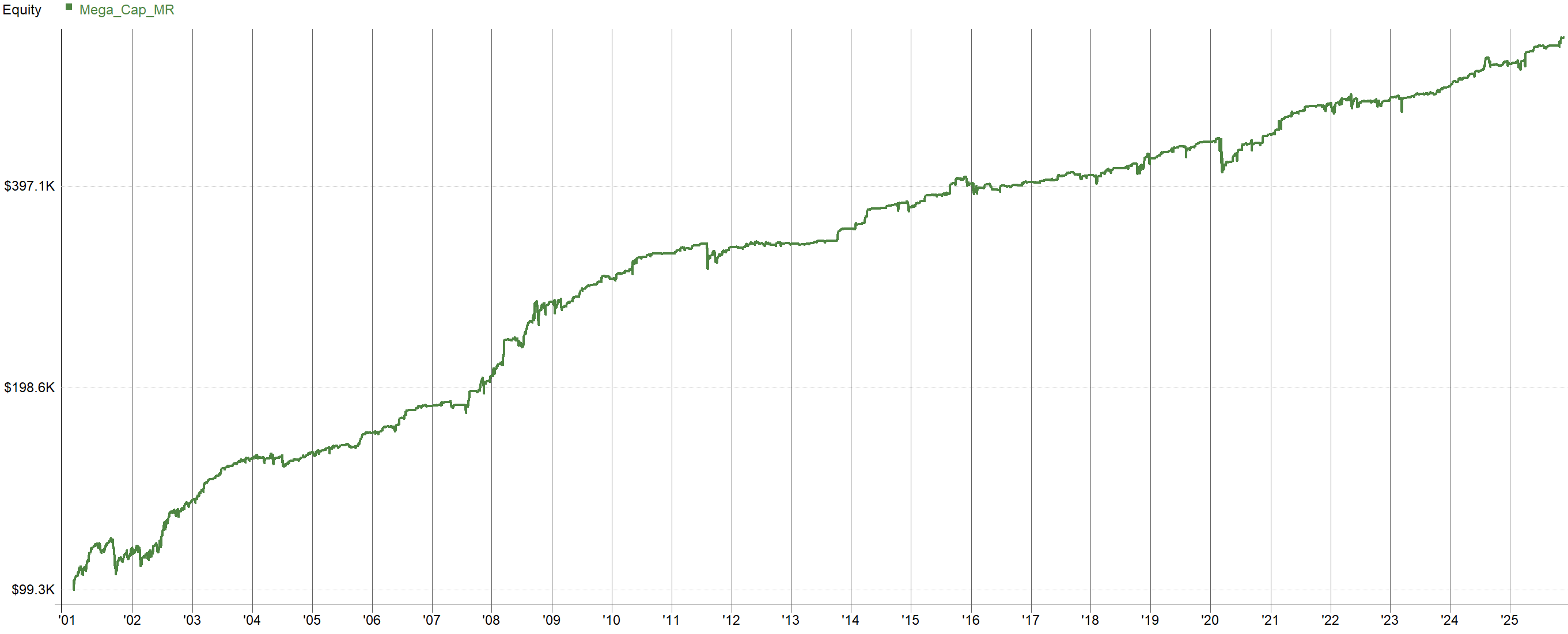
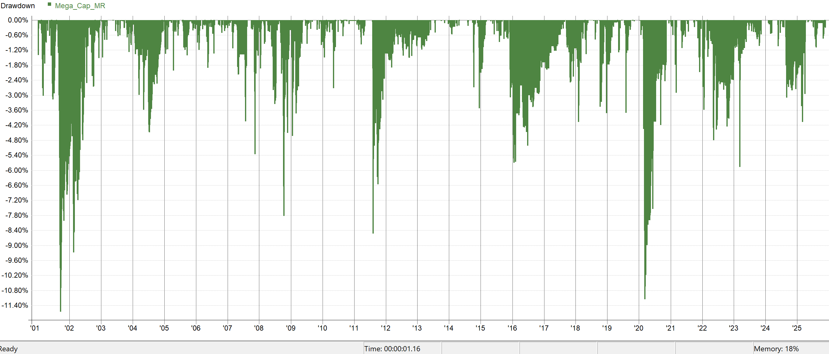
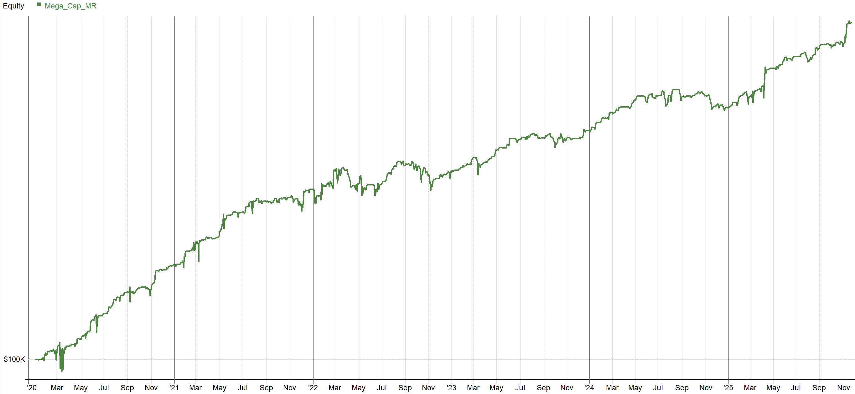
As a refresher, this is the current result of the system we are working with:

Alright, let’s dive in and see where this system shines and where the system has flaws. Ultimately, we need to decide if the system is worthy of the portfolio or not. So, let’s begin some robustness tests!
Parameter Sensitivity:
The first robustness test to assess is a parameter sensitivity. If you remember from the part 1 article, I ran a parameter sensitivity on the in-sample. Now, I want to run the same parameter sensitivity on the out-of-sample. I want to focus specifically on the out of sample because I want to understand a couple things:
Is the out-of-sample time period more “fragile” or sensitive to parameter values than the in-sample?
Did the out-of-sample get “lucky” in terms of positive performance
It’s 100% possible to have a lucky out-of-sample result that only had positive performance due to shear luck. The parameters chosen in the system could be on an out-of-sample performance peak and just happened to make money during the out-of-sample period. But going forward in time, that performance peak will eventually collapse or shift, leading to poor or negative results. This is what we want to check for.
Hence, I ran a +-25% parameter variation on all parameters within the system, specifically on the out-of-sample time period. The table below shows the percentile the default system parameters reside in terms of performance.

For all metrics, the system was basically right in the middle of the road, in fact the system performance was slightly less than the average result. The only exception was Percent Wins being 67%, but for all other metrics, the system was below the 50th percentile.
Assuming all results within the +-25% parameter space are positive, this is exactly what you want to see. You do not want the systems default parameters to be in a super high percentile. That would be evidence of selecting a performance peak that just hasn’t shifted yet, i.e. a lucky out-of-sample result.
The fact that this system is in the middle of the road basically means as the optimal parameters shift around over time, this system is right in the middle of the road and has the wiggle room to handle the noise in the parameter surface.
Visualize it this way, it’s much easier for a new driver to drive a car down the middle of the road than right on the edge. When driving down the middle of the road, there is plenty of room on either side to account for the new drivers poor driving skills. When driving right on the edge of the road, one side has no margin, one wrong move and the car is in a ditch. Kind of a dumb analogy, but that’s how I think about it.
Now, let’s compare some of the results from this +-25% optimization. I’ll show the default system parameters out-of-sample performance first, then I’ll show the best and worst results in terms of Calmar ratio (ROR/MaxDD).
Default Parameters Out-of-Sample:
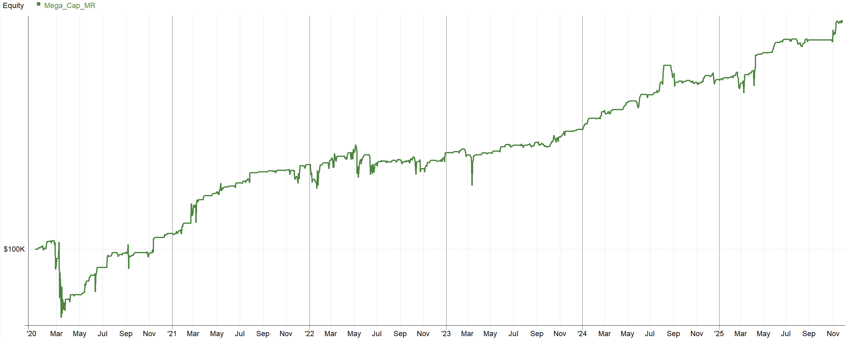

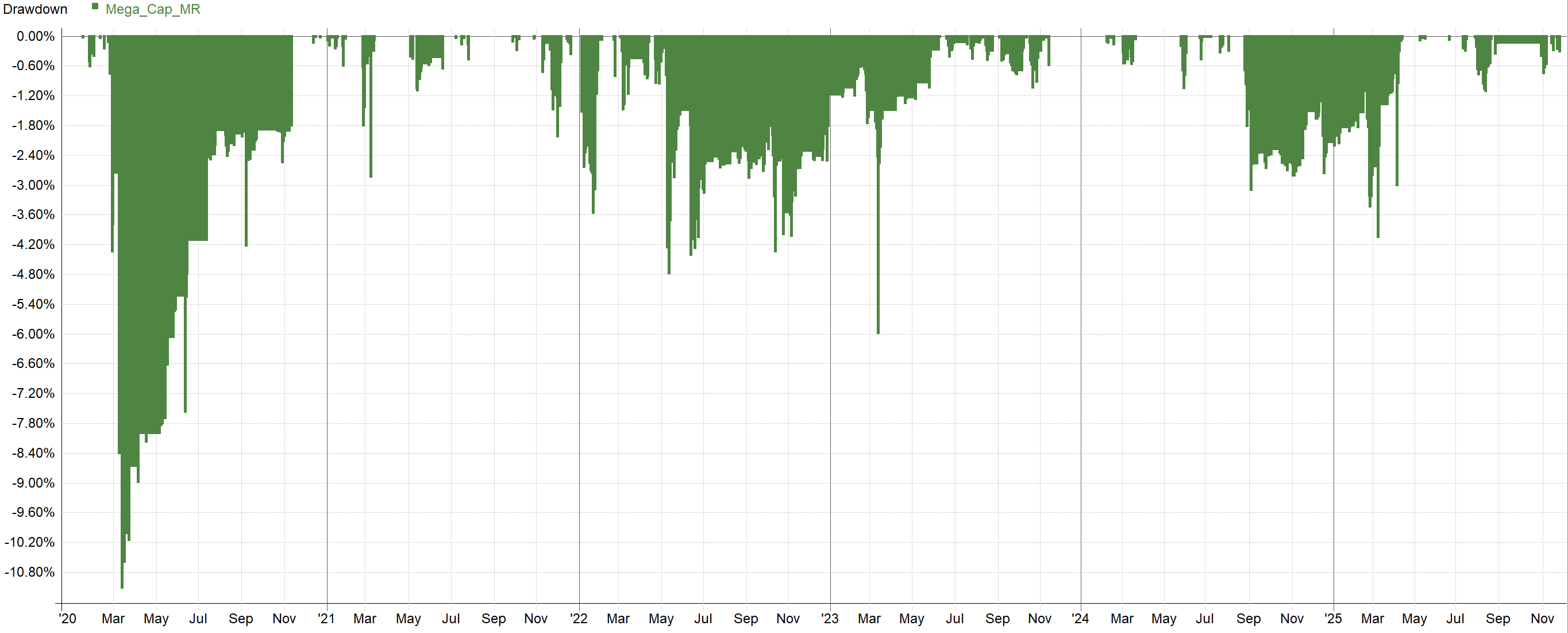
Next I’ll show the equity curve of the best result in terms of Calmar ratio from the +-25% optimization.
Best Result (Based on Calmar Ratio):

You’ll notice this parameter set happened to miss Covid, then go on a steep upward slope, making new high after new high. It’s good to see results significantly better than the default parameter set.
I would never complain if the parameter surface shifted in this direction and the default parameter system started seeing performance like this. If the markets shift and the default parameters start performing better than they do currently, it’s nice to see this type of performance is possible.
Worst Result (Based on Calmar Ratio):
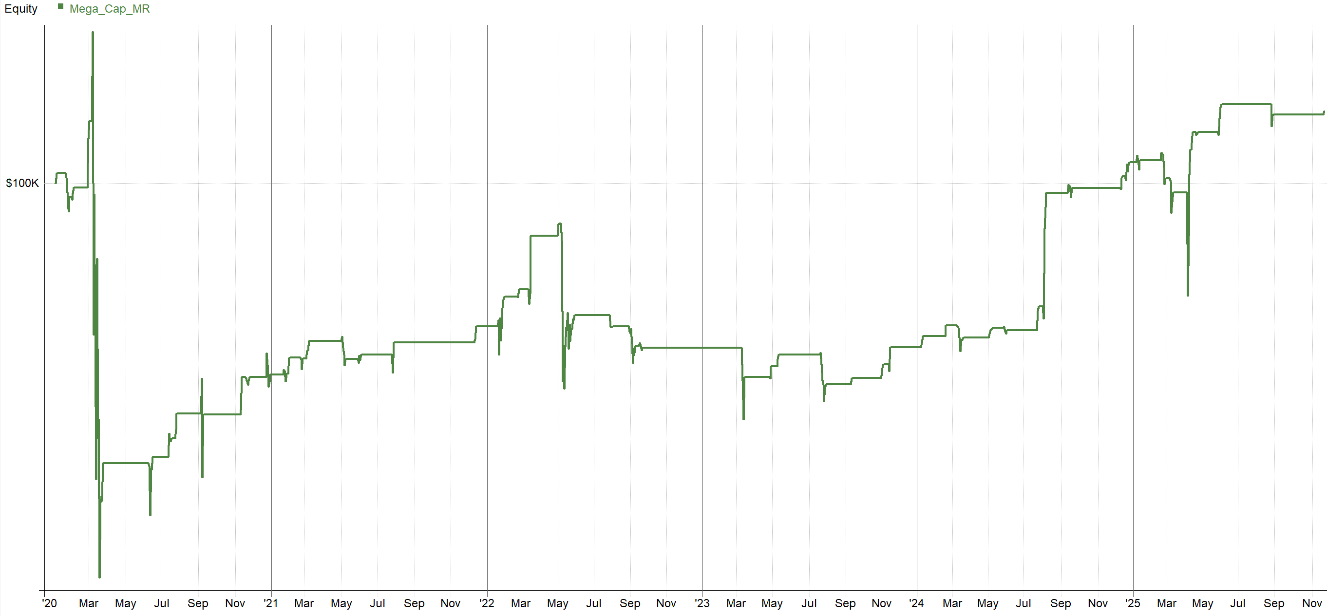

Above is the results of the worst equity curve based on Calmar ratio. You’ll notice these results have very few trades (125 vs. the default systems 580). Basically this parameter set within the +-25% range is choking the system performance. The oversold measuring parameters become very low, and the ADX parameter is very high, leading to a very restrictive set of conditions which would result in a trade. Basically, this was the most stringent possible parameter set within the +-25% results.
On one hand, this is an ugly result. On the other hand, even though this variation of the system had an overly strict parameter combination, the system still worked its way up and to the right. This is a good sign that even under very stringent scenarios, the system rules still resulted in a positive outcome.
Let’s now check out a more realistic worst case result from the +-25% parameter variation. The above parameter set only had 125 trades during the out-of-sample period while the default parameters have 580 trades. Let’s again sort the results of the +-25% parameter variation by the worst Calmar ratio, but check out a system with slightly more trades, say 350 trades. This will let us see the results of a “poor performing” parameter set that does not choke the system.
Realistic Worst Result (Based on Calmar Ratio):
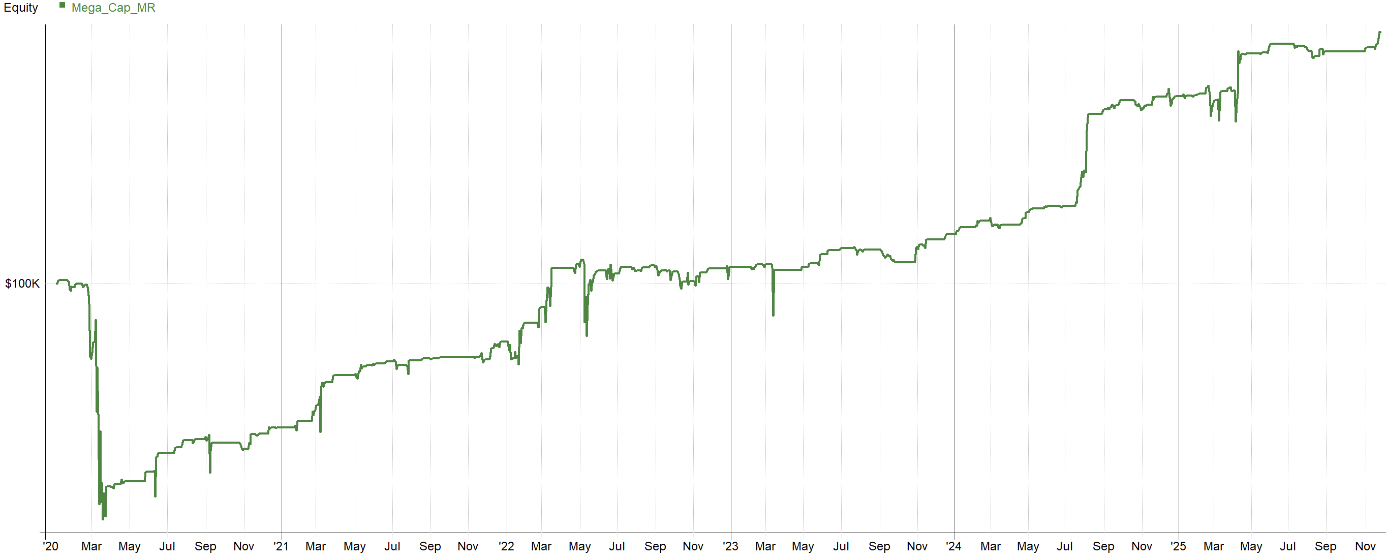

Okay, this parameter set had 349 trades, close enough to 350. As you can see, with a parameter set that is not as restrictive, even the results on the worse end of the +-25% parameter variation are pretty good. I would trade this parameter set, even though it’s in the bottom 4% of parameter values in terms of Calmar.
Overall, the out-of-sample +-25% parameter set variation shows promising results. The system appears to be in a very stable range of parameters which is exactly what we want to see. All +-25% parameter variations make money in the out-of-sample time period and every equity curve that has a reasonable number of trades is profitable and tradable.
Entry Rule Monte Carlo:
A neat Monte Carlo you can run to test the systems ability to choose good trades is via Entry Rule Monte Carlo. I’ve seen many systems fail this test which is why I like this test a lot.