All Weather Portfolio Research: Part 2

Three TradeQuantiX All Weather Portfolio Versions

In the last post about All Weather portfolios we looked at a bunch of different All Weather portfolio ideas. We coded up 9 examples of All Weather portfolios found online and figured out what we liked and didn’t like about them. In this article, I am going to take this one step further and create my own All Weather portfolios. I will show a total of three variations of an All Weather portfolio. One variation will have a static allocation that is only rebalanced monthly (quarterly, semi-annually, yearly etc. rebalance intervals is also possible), another variation will be a tactical asset allocation with specified fixed allocations to each asset, and the third will be tactical allocation with volatility targeted position sizing. Let’s jump in.

If you remember from the previous article, there were a lot of things I did not like about the All Weather portfolio I explored. One of the things I did not like was many of these portfolio equity curves just looked like SPY with less returns. I want to try to develop an All Weather portfolio that has a more unique and uncorrelated performance profile to SPY. Another thing I did not like was most of the All Weather portfolios broke or underperformed in 2022. Something changed in the markets that caused many of the All Weather portfolios assets to become positively correlated. The All Weather portfolio I want to make needs to have more diversification, so that it can better handle situations like 2022.

To create a better All Weather portfolio that can conquer more market conditions and have uncorrelated returns to SPY, we need to start by having more ETFs in the portfolio. These ETFs need to represent different asset classes that are generally uncorrelated in nature. These ETFs should not just be chosen because they have performed well historically. In fact, historical performance if an ETF was not considered when creating this list of ETFs. I started by thinking of the most intuitively uncorrelated things that were in ETF form, starting with many of the ETFs used in the part 1 of this article series, then expanding from there. To get a stable return in any environment, we need uncorrelated ETFs. A summary of the final ETFs I have considered for this All Weather portfolio are:

• QLD (2x QQQ Nasdaq 100)

• GLD (Gold)

• TLT (20+ Year Treasury Bonds)

• SHY (1-3 Year Treasury Bonds)

• XLE (Energy Sector)

• DBC (Commodity Index)

• DBA (Agriculture Commodity Index)

• VEU (Global Equity Excluding USA)

• XLP (Consumer Staples Sector)

• IYH (Healthcare Sector)

• VNQ (Real Estate Index Fund (REIT))

• BITO (Bitcoin ETF → GBTC used in backtests due to longer price history)

• UUP (US Dollar Index)

If you have other ETF ideas, let me know, let’s add them, the more the merrier. A correlation matrix of the returns of the ETFs listed above looks like the following:

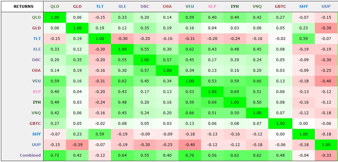
There are a vast range of correlations in this table. Many of the correlations are at 0.5 or below, with many correlations being negative. The goal of this All Weather portfolio is to have as many non-correlated ETFs as possible to survive times of market volatility and uncertainty. While many ETFs are uncorrelated, some ETFs are relatively correlated, like VNQ and VEU, but even those are only at a 0.66 correlation. Granted 0.66 is considered a somewhat strong correlation, but considering VNQ are REITs and VEU is Global Equities they are fundamentally different assets. So even though the correlation may we somewhat strong, I am using intuition to say there may be times on the future where these ETFs are significantly uncorrelated and may help the overall portfolio. Analysis and numbers are not everything, sometimes intuition gets a say in the analysis.

Some may argue that using intuition to determine what to add to an All Weather portfolio is non-sense, but let me take the example to the extreme to illustrate a point. Assume I had two ETFs that were very strongly correlated over ten years. Say one ETF was for cattle prices and the other was for government bonds. I highly doubt those two assets have any real direct connection in prices to each other. Now assume in that ten year time frame the whole economy was booming and everything was increasing in value. If that is the case, then these two assets would probably be positively correlated because everything was going up. That doesn’t mean the two assets are intrinsically linked in their movements. That example is exactly what has happened the US economy the past 14 years. We have had a massive bull market, so of course a lot of assets are going to go up, leading to a positive correlation, but correlation is not causation and does not mean assets are intrinsically linked. This is why even though some ETFs representing an asset are somewhat correlated, they were still added to the portfolio.

Here are some assumptions that apply to each of the three All Weather portfolios we will explore. Each of the three All Weather portfolios will use the same list of ETFs, but the way the system works will be different. Each system will rebalance or reallocate on the first of each month. Each test will be from 2000 to today (2024). Some ETFs did not exist in the very beginning of the backtest, so performance during the first few years may be misrepresented. By 2007 all ETFs were available except GBTC (which was available starting in 2015). No leverage was used in any of these tests. Let’s begin.

(Note: Below I show three All Weather portfolio variations. As I was editing this article I realized there was one more All Weather portfolio variation I wanted to explore as well. I figured this article was getting long so there will be a part 3 article where I explore a fourth All Weather portfolio variation.)

TradeQuantiX All Weather Portfolio 1 (Static Allocation):

Using the ETFs listed above, we can create a pretty simple and straight forward All Weather portfolio. Basically, just buy and hold all of those ETFs forever. From there, we can either rebalance the portfolio from time to time (Monthly, Quarterly, Semi Annually, Yearly etc.) or never rebalance. Rebalancing after a year or longer will be the most tax efficient, but waiting that long to rebalance may cause the ETF weightings to get too far out of wack. More frequent rebalancing will keep allocations in check, which will likely create a smoother equity curve, but be less tax efficient. It’s really the preference of the investor, so I will show a couple variations of rebalance timing.

The other thing to consider is do we give each ETF an equal weighting or do we vary the allocations depending on the ETF? For example, it probably doesn’t make sense to give bitcoin and equities the same weightings. The volatility of Bitcoin is significantly higher than equities, giving both assets the same allocation would result in a very volatile return, the exact opposite of what we are trying to achieve. So, what I will do is give a “common sense” allocation to each asset class based on historical volatility. Therefore, each ETF will have a similar contribution to overall portfolio returns and volatility. One problem is some of these ETFs will have such a low volatility, so in order to make them equally contribute to the portfolio you need a massive position size. Since this is the real world and we are constrained by not having infinite money, I have capped an individual ETF allocation at 10% because we don’t want too much money in any one ETF; and 10% seems like a sensible number. Too much allocation to any one ETF increases the risk of the portfolio, if that ETF drops 50% and there is a high allocation to it, that’s going to hurt. We want to minimize ETF specific risk and diversify, that’s one of the purposes of an All Weather portfolio.

To determine the static allocations for each ETF, I calculated the volatility of each ETF for every year from 2010 to 2024 and averaged the results. Then I found the allocation required to give to each ETF such that they contribute equally to the overall portfolio. Then I capped any individual allocation at 10% and scaled the remaining allocations up until exposure summed to 100%. Those allocations are shown in the table below:

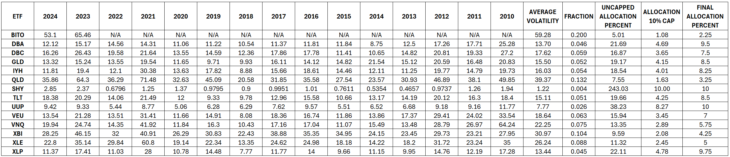
• Table Column Definitions:

  • AVERAGE VOLATILITY: the average one year volatility of the ETF.

  • FRACTION: the ETFs contribution of volatility with AVERAGE VOLATILITY normalized to 1. So assuming equal weight allocation, this is the contribution the ETF would have to portfolio volatility.

  • UNCAPPED ALLOCATION PERCENT: 1/Fraction

  • ALLOCATION 10% CAP: min(UNCAPPED ALLOCATION PERCENT, 10%)

  • FINAL ALLOCATION PERCENT: ALLOCATION 10% CAP scaled up (still capping at 10%) until all allocations sum to 100% (rounded to the nearest 0.25%)

Over time, the volatility of an ETF may change, so the position size may need to be updated in the future. Some of the ETFs have vastly different volatility from year to year, so this approach is not perfect, but it is simple and effective. I should note, with this first All Weather portfolio example, I am tailoring it to the passive investor. This All Weather portfolio is built for the person who does not what to do a lot of work, they just want to buy these ETFs and let the portfolio grow with minimal intervention. This is why I took this simple volatility approach to determining sensible allocations, it’s not perfect, but it’s what I would call an 80% solution (referring to the 80/20 rule, the Pareto Principle).

One drawback of the approach I used to determine allocations is I used all the data to make the allocation decisions, which isn’t ideal. My allocations used in say 2010 are influenced by years 2011 to 2024, which have not occurred yet. To avoid this future leak, you could just used fixed fractional position size (all positions are the same size), but this will likely result in more volatile results. Or you could do a rolling allocation where the allocation is readjusted every year based on the average of the previous years volatility, but this adds complexity that a passive investor may not want to worry about. In the third All Weather portfolio, I will address this allocation issue, so no need to worry we are building our way there, though the solution is a little more active than this first All Weather portfolio.

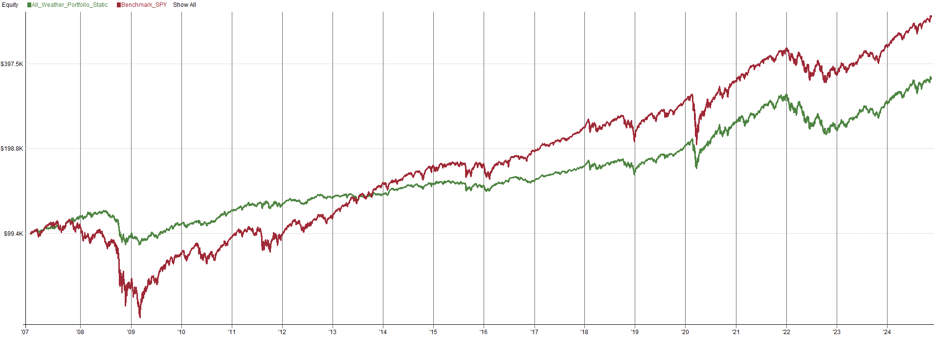
Now, let’s take a look at the first All Weather portfolio historical performance. Remember this portfolio holds 13 ETFs, rebalances monthly, and uses a static allocation based on the average ETF volatility.

Rebalance Timing: Monthly

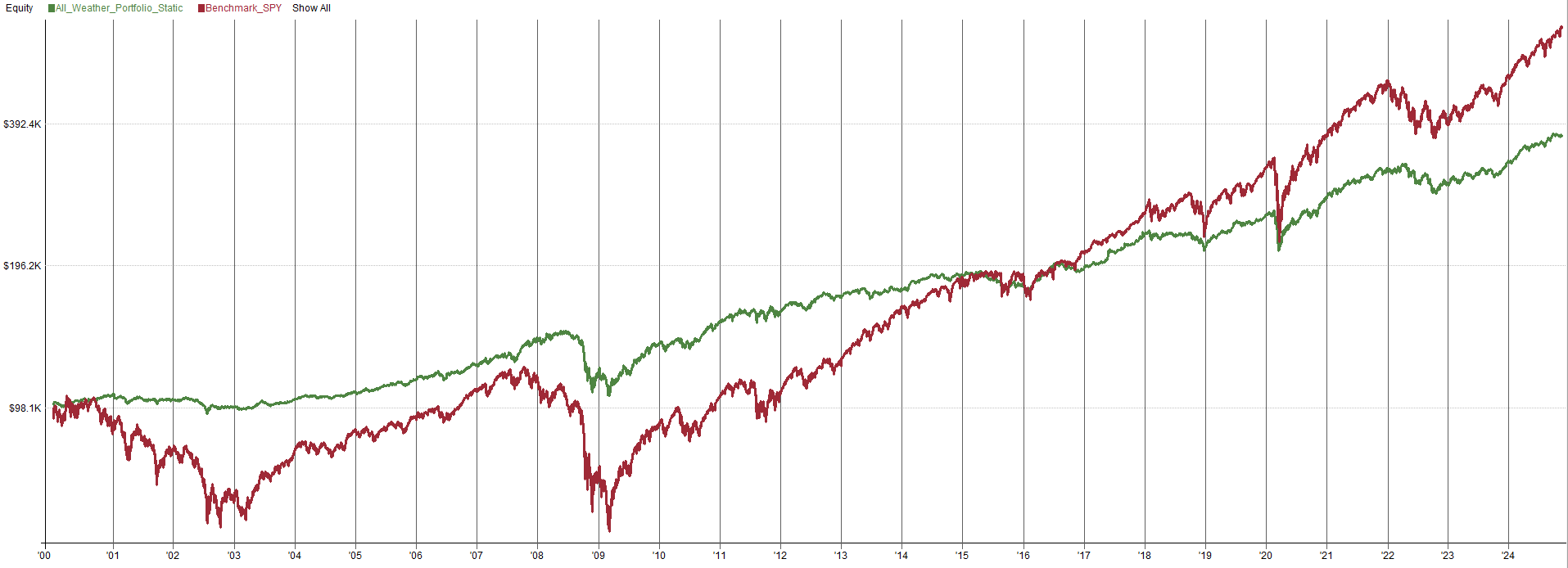
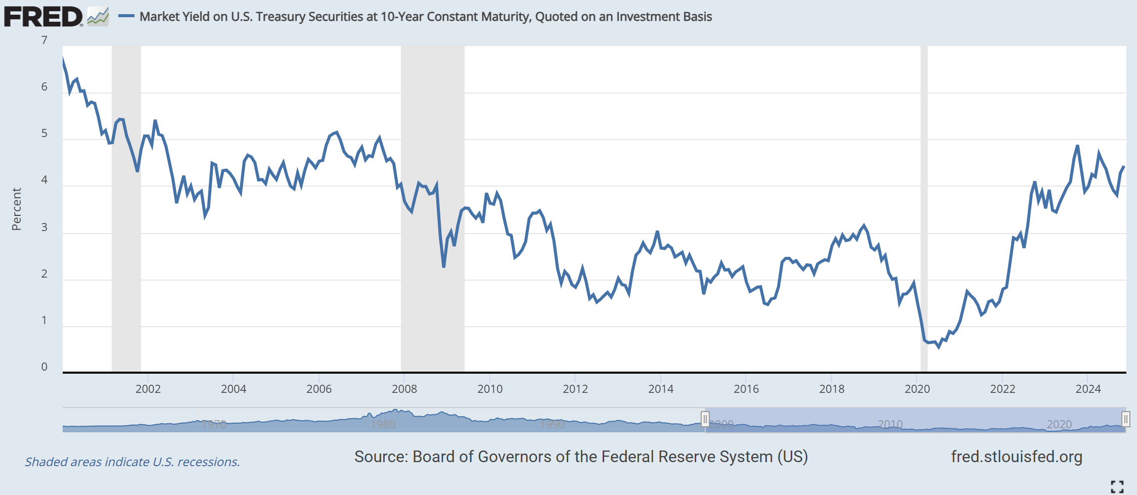
Honestly those results are not too bad. 2008 kind of sucked, but it sucked less than the SPY ETF. Other than 2008 the results are relatively stable, consistent, and low volatility. Risk adjusted, this beats the SPY ETF during the backtest period. For a low risk passive investor, this may be a good portfolio solution. The returns are only 5.40%, which isn’t terrible, but if the risk free rate increases then it may make more sense to just invest in the risk free rate. Though from the year 2007 onward the risk free rate was less than the return of this All Weather portfolio. So keep in mind if the risk free rate goes back above 5.4%, then this All Weather portfolio is not that great anymore.

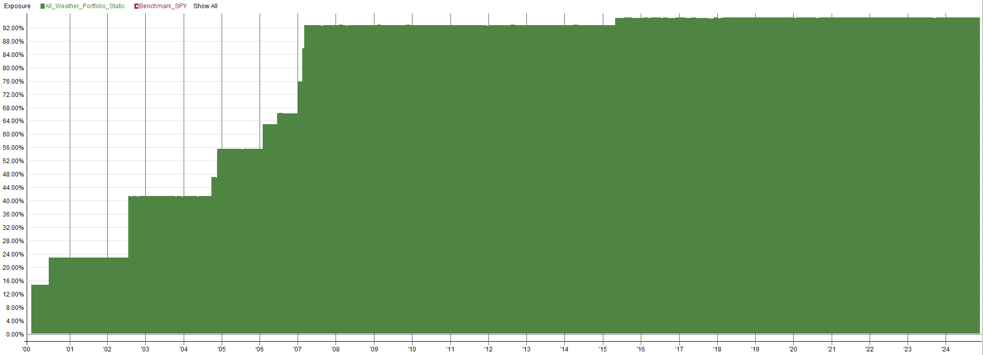
One thing to note, notice how the exposure ramps up over time. Not all of these ETFs were available when the backtest started in 2000. As ETFs become available, the system can start buying them, but the first 7 or so years of the backtest may be misrepresentative because it would have only been invested in a few of the ETFs (meaning the portfolio was underexposed, lowering returns and drawdown). From 2007 onwards would be more or less representative.

Now let’s consider this same portfolio with quarterly rebalancing. This would make the portfolio even simpler to implement, only needing intervention four times a year.

Rebalance Timing: Quarterly

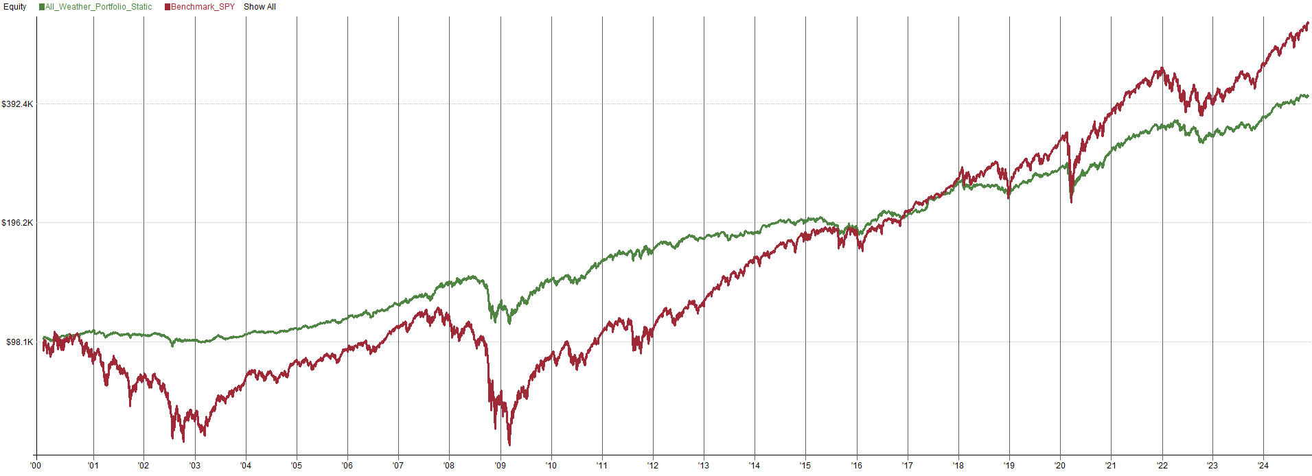
Now let’s make this portfolio even simpler an rebalance once a year on the first trading day of the year. This is efficient from a tax perspective as you could take advantage of long term capital gains tax as opposed to short term capital gains tax applied to positions held for less than one year (this applies to US tax residents, I am not sure how other countries handle taxes on capital gains).

Rebalance Timing: Yearly

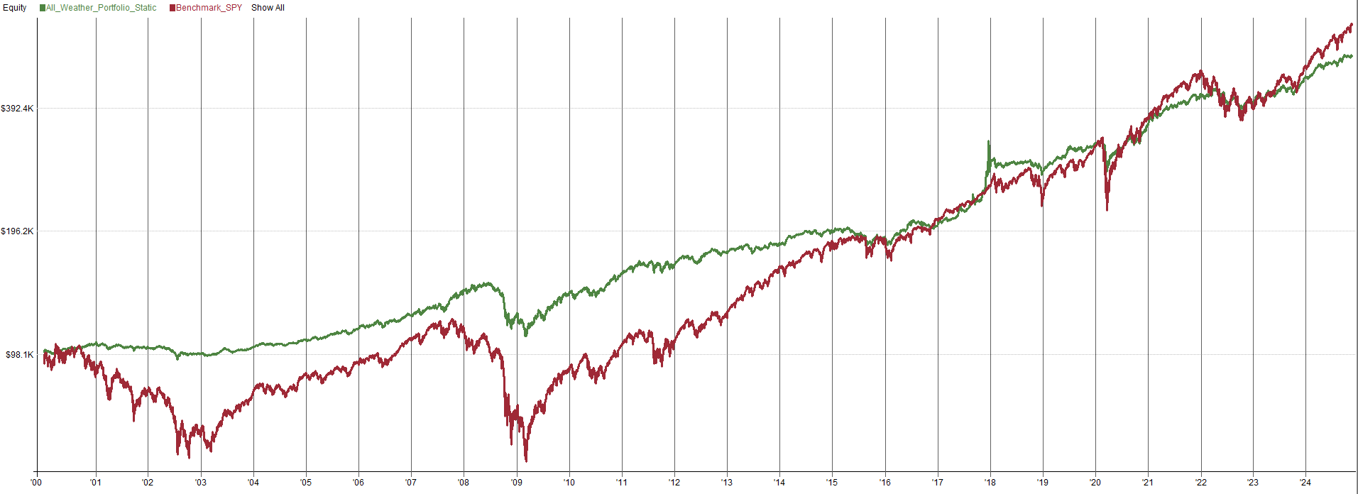
You can start to see the impact of infrequent rebalancing. In 2017 Bitcoin volatility goes crazy and the portfolio returns become denominated by Bitcoin, until the rebalance happens at the start of 2018. The longer the timeframe in-between rebalancing, the more subject you are to ETF specific risk and you can drift away from a fully diversified portfolio (since one highly volatile ETF can begin to dominate performance if not rebalanced).

Finally, here is an example of never rebalancing. The test is started in 2007 because this is the year where all ETFs (except bitcoin) become available. If I started this backtest in 2000 like the others, the ETFs available first would have up to 7 extra years to accumulate returns before the rest of the ETFs were invested, this would skew the results for this test since we never rebalance.

Rebalance Timing: Never (With Bitcoin ETF)

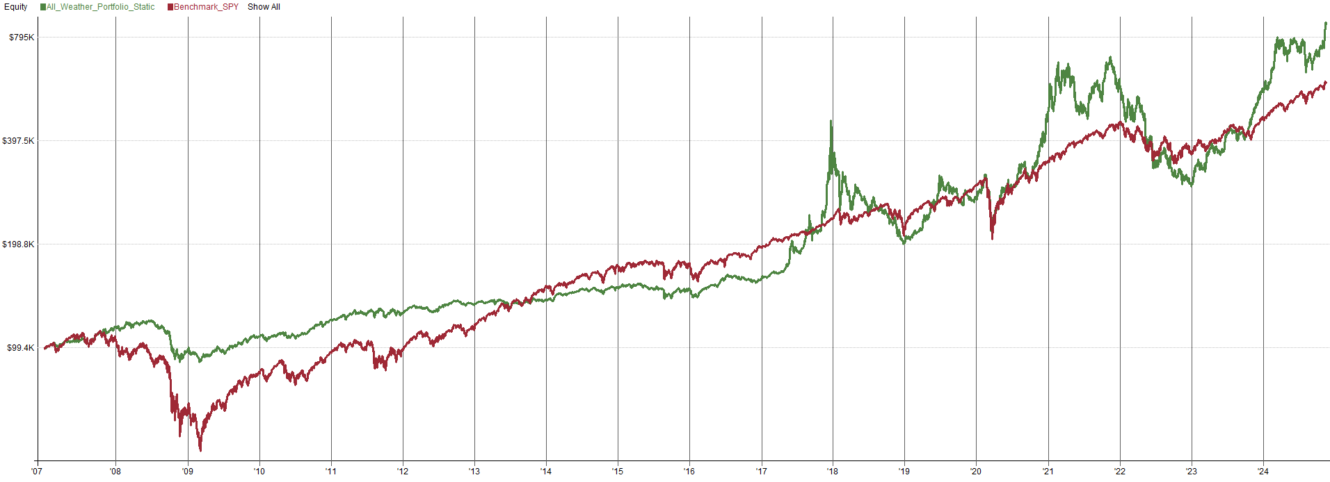
Here you can see the benefit of rebalancing. The effect of Bitcoin becomes massive and the portfolio basically becomes a buy and hold Bitcoin rather than an All Weather portfolio. Rebalancing is definitely important, especially when the portfolio holds assets with very different volatilities. I decided to take Bitcoin out of the portfolio to see what happens since it was skewing the results.

Rebalance Timing: Never (Without Bitcoin ETF)

By the end of the 26 year period, the return profile looks like buy and hold equities. That is because equities have done well over this timeframe, so they have accumulated a large position within the never rebalance version of this portfolio. This defeats the purpose of an All Weather portfolio, we should have a return profile that is smoother and somewhat uncorrelated to the equities market. Never rebalancing seems unreasonable to me.

This first All Weather portfolio may or may not be very exciting to you. You may be looking for more returns because 5.4% seems boring. You may be thinking “I bet if I optimize those allocation fractions and remove the poor performing ETFs I can boost the returns of this portfolio”. That is very dangerous and called curve fitting. Just because you can make something perform well historically does not mean that performance will continue into the future. Past optimal allocations are not indicative of future optimal allocations as the future is never the same as the past. I could definitely make this All Weather portfolio look better in a backtest, but it’s curve fit and full of hindsight bias.

The returns of a curve fitted backtest will look nice, but will it perform into the future? Maybe, but most likely not. We need a better way of creating an All Weather portfolio. Yes, a static All Weather portfolio will be better from a tax perspective and is the simplest to implement; but if you are interested in getting returns greater than the market then we need to use a different method than optimize allocations or cherry pick ETFs. Hence, I have two more All Weather portfolios to show you.

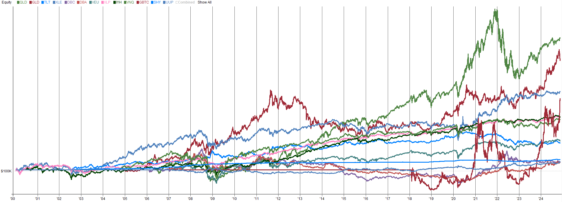
This first All Weather portfolio did not cherry pick ETFs based on performance nor did it optimize allocations, so the performance is likely real, which is why the performance isn’t amazing, but it also isn’t bad (it’s all relative to your own objectives). So how can we improve the system without introducing too much optimization or cherry picking? First off, we will stick with the same ETFs, and if we find more non-correlated ETFs in the future we will add those to the All Weather Portfolio as well. Second, we need to introduce tactical asset allocation. Basically, this is a simple on/off switch which will be used as a way to say “yes, own this ETF now” or “no, sell this ETF now”. The simplest on/off switch I can think of is own the ETF if it is above its 200 day moving average and don’t own the ETF if it is below its 200 day moving average. I did not optimize this rule, I did not cherry pick this rule, it’s just a very simple way to define an uptrend vs. downtrend. So the next two versions of the All Weather portfolio will use this logic in the system, thus only ETFs in an uptrend are owned by the All Weather portfolio. Below is an image of all the ETFs price performance in the All Weather portfolio:

The next image is all the ETFs in the All Weather portfolio where the ETF is only owned above its 200 day moving average.

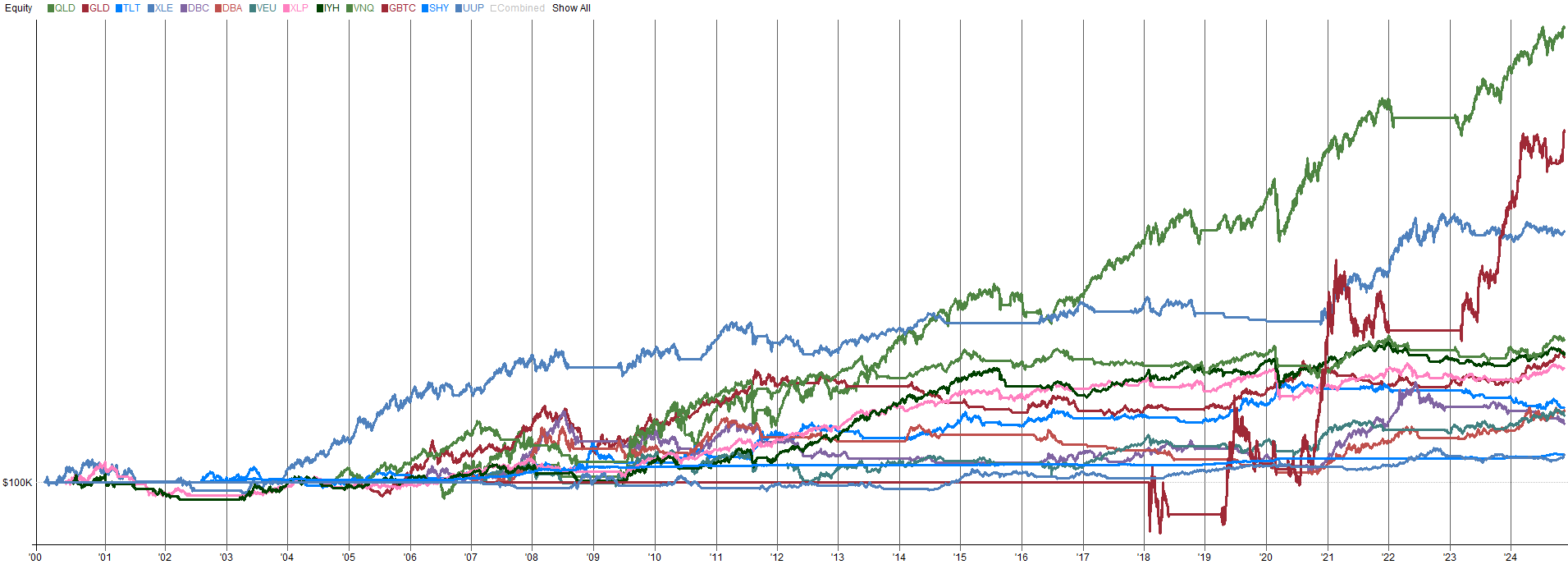
I’m a visual person, so this helps me see what’s going on. Visually, I see less downside and smoother price action with this on/off switch. I think you could imagine how a long only All Weather portfolio would benefit from only owning ETFs in an uptrend. So let’s jump into this concept with our second All Weather portfolio.

TradeQuantiX All Weather Portfolio 2 (Tactical Asset Allocation with Fixed Position Sizing):

As briefly introduced in the previous section, we are going to take our static All Weather portfolio and convert it to a tactical asset allocation All Weather portfolio. Rather than owning all ETFs at the same time, let’s use a simple market timing switch determine when we own or don’t own an ETF. The timing switch says to own the ETF if the close is above the 200 day moving average and don’t own the ETF if the close is below to 200 day moving average. We will rebalance based on the same allocations from the first All Weather portfolio monthly. This means the market timing switch will only be checked monthly as well. So on the first of the month the All Weather portfolio will check all the positions and buy the ETFs that are above the 200 day moving average and sell any ETFs in the portfolio that are below the 200 day moving average. All other ETFs that are owned but not sold will be rebalanced on the first of the month.

The tactical asset allocation All Weather portfolio will use the same volatility based fixed position sizes as the first All Weather portfolio. This prevents any one ETF from dominating the return profile because its volatility is higher than the rest of the ETFs. It will also serve as a back-to-back to the static allocation All Weather portfolio, so you can see the power of the simple market timer.

The tactical asset allocation All Weather portfolio is a little more complex than the static allocation All Weather portfolio. Granted, the complexity is one rule, only own the ETF if it’s above the 200 day moving average, so really it’s not that bad. You could argue that tactical asset allocation method will be less tax efficient since it is rebalancing and buying/selling ETFs monthly, but if you were to rebalance the static All Weather portfolio monthly then in reality it wouldn’t be that different. One of the pros of tactical asset allocation is we own the well performing ETFs and sell the laggards. So, tactical asset allocation is essentially a dynamically adjusting All Weather portfolio. It’s an All Weather portfolio that actually adjusts to the market conditions; which if you think about it, that’s kind of what you want with an All Weather portfolio. If 10 of the 13 ETFs are going down, why would I want to own those? I want to own the 3 ETFs that are performing well in the current market environment.

So let’s take a look at the performance of the tactical asset allocation:

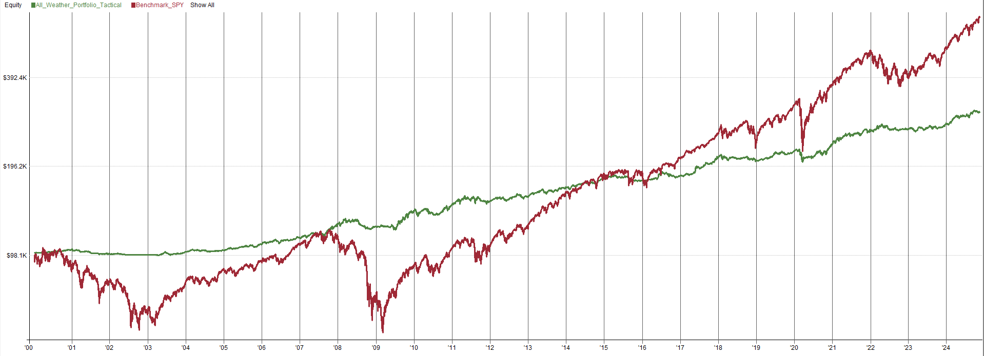
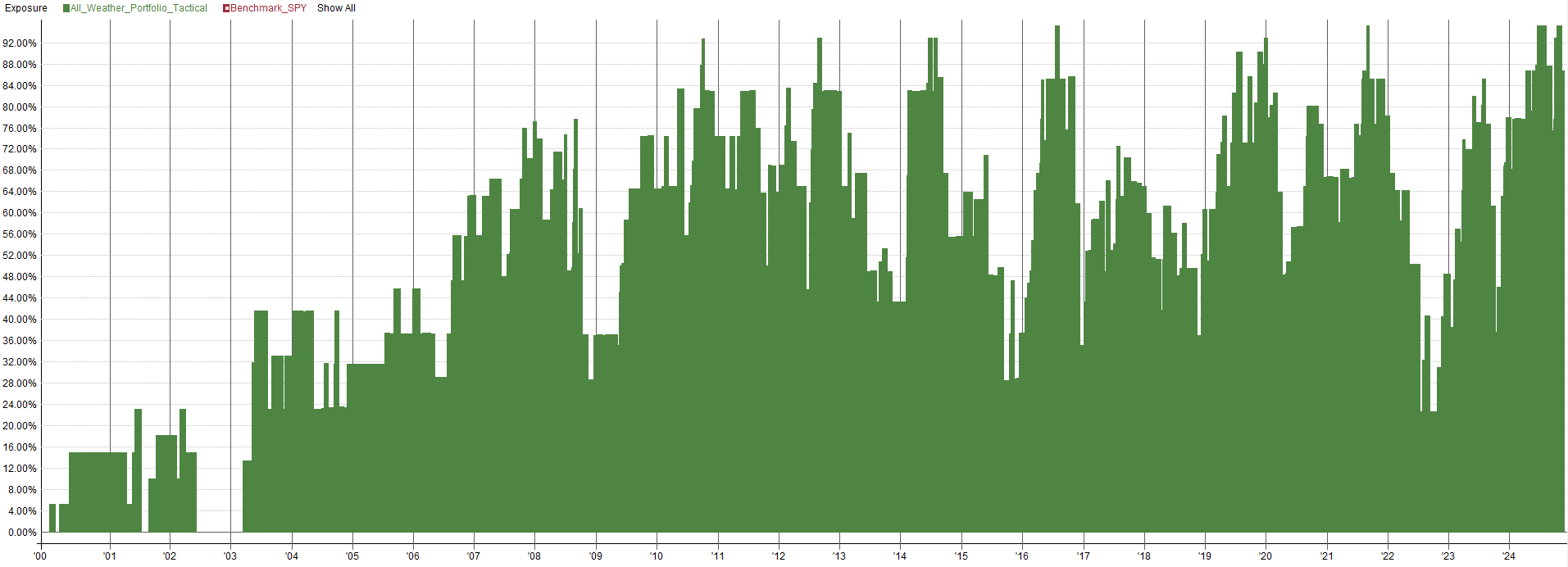
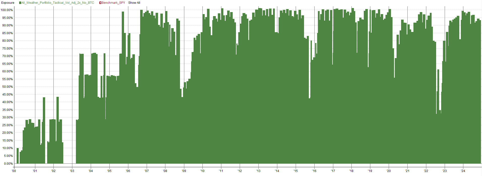
As you can see, the system is extremely low volatility, low drawdown, but also low returns. The equity is very stable over time, as the volatility based position sizing ensures all ETFs contribute a similar volatility to the overall portfolio. Since these ETFs are somewhat uncorrelated, this provides a smoother ride along the equity curve. From the exposure plot (calculated as the percentage of total capital invested in the market), the system is mostly under exposed for the entire duration of the backtest. To increase returns, we need to find a way to bump up our average exposure over time. This is where a modification of this All Weather portfolio will come into play.

In an attempt to increase our exposure to the markets over time to boost returns, we will approach capital allocation a little differently. This time, we will take our ETF allocation percent and multiply by 1.5. This would create leverage, so to avoid that, let’s add an exposure constraint to say exposure needs to be capped at no more than 100% (no leverage). In doing this, we may not be able to hold every ETF anymore, we may only be able to hold 7 to 8 at a time. This will cut back on diversification a little but, but will boost returns and honestly, you’re still fairly well diversified with 7 to 8 ETFs. The performance with the boosted position sizing can be seen below:

Now, you can see exposure is near 100% for the majority of the backtest. The compounded annual growth went from 4.51% to a more respectable 6.54%, and the drawdown is still low at 13.43%. Not too bad. The system survives 2008, 2022 is just a flat spot, and the 2020 Covid crash is about 1/3 the drawdown that SPY experienced. That’s pretty good for such a simple system! But we can do better. We still have one more All Weather portfolio to look at, which will take this process one step further and again improve performance all around. So let’s get to it!

TradeQuantiX All Weather Portfolio 3 (Tactical Asset Allocation with Dynamically Adjusted Position Sizing):

On to the third version of our All Weather portfolio. This one will build on the previous two portfolios we have examined. This third All Weather Portfolio will be a tactical asset allocation just like the second All Weather portfolio. The only upgrade is the position sizing will be recalculated with every entry, rather than having a fixed allocation associated with each ETF. The position sizing will be calculated based on recent volatility so each ETF contributes the same volatility to the overall portfolio. Thus, if the volatility changes over time, this third All Weather portfolio will be able to handle volatility changes with updated position sizing calculations. Let me specify the rules more closely below:

• System rebalances and buys/sells positions monthly, on the first trading day of the month

  • New ETFs are entered if they are now above the 200 day moving average, position sizing is calculated based on volatility

  • Any previously owned ETFs are sold if they are now below the 200 day moving average

  • Positions that have been held since last month and do not have a sell signal get rebalanced based on volatility

• Up to 10 ETFs can be held at once

• If more than 10 ETFs meet the entry criteria, rank them based on momentum:

  Ranking = ROC(C, 120) + ROC(C, 60) + ROC(C, 30)

  • ROC stands for Rate of Change

• Calculate the ETF volatility:

  • ETF volatility calculated based on the average of 5, 20, and 100 day lookbacks.

    ForcastedVol = (StdDev(ROC(C, 1), 5)*SQR(252) + StdDev(ROC(C, 1), 20)*SQR(252) +  StdDev(ROC(C, 1), 100)*SQR(252)) / 3

• Calculate the position size based on ETF volatility (position size calculated in shares):

  • If the volatility based position sizing exceeds 10%, cap the position size at 10% to prevent very low volatility ETFs from consuming all our capital.

    PositionSize = Min(CurrentPortfolioEquity * DesiredVolatility/ForcastedVol/Close, CurrentPortfolioEquity/10/Close)

When we put all that together we end up with a tactical asset allocation All Weather trading system with dynamically adjusting position sizes. Really, the only part of the system that is somewhat complex is the position sizing. Other than the position sizing, there is one entry and exit rule (C>200 day MA) which is evaluated on the first trading day of every month. Overall, the system is simple, yet effective. So now we can check out the performance of the third All Weather portfolio:

Hey that looks pretty good! 6.33% returns with 11.13% drawdown, that way out performs any of the traditional static All Weather portfolios we looked at in the part one of this article series. Some may say 6% return isn’t that impressive, but that comes with only an 11% drawdown. On the other hand the SPY had a drawdown of over 50% in the 2008 financial crisis. Risk adjusted, this third All Weather portfolio destroys the performance of the SPY.

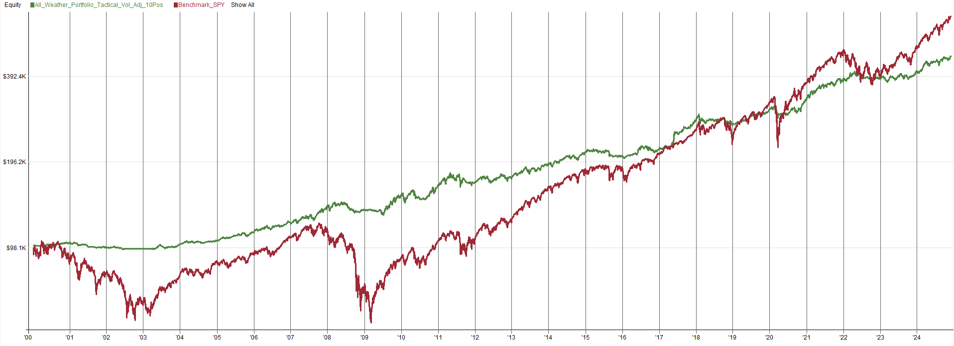
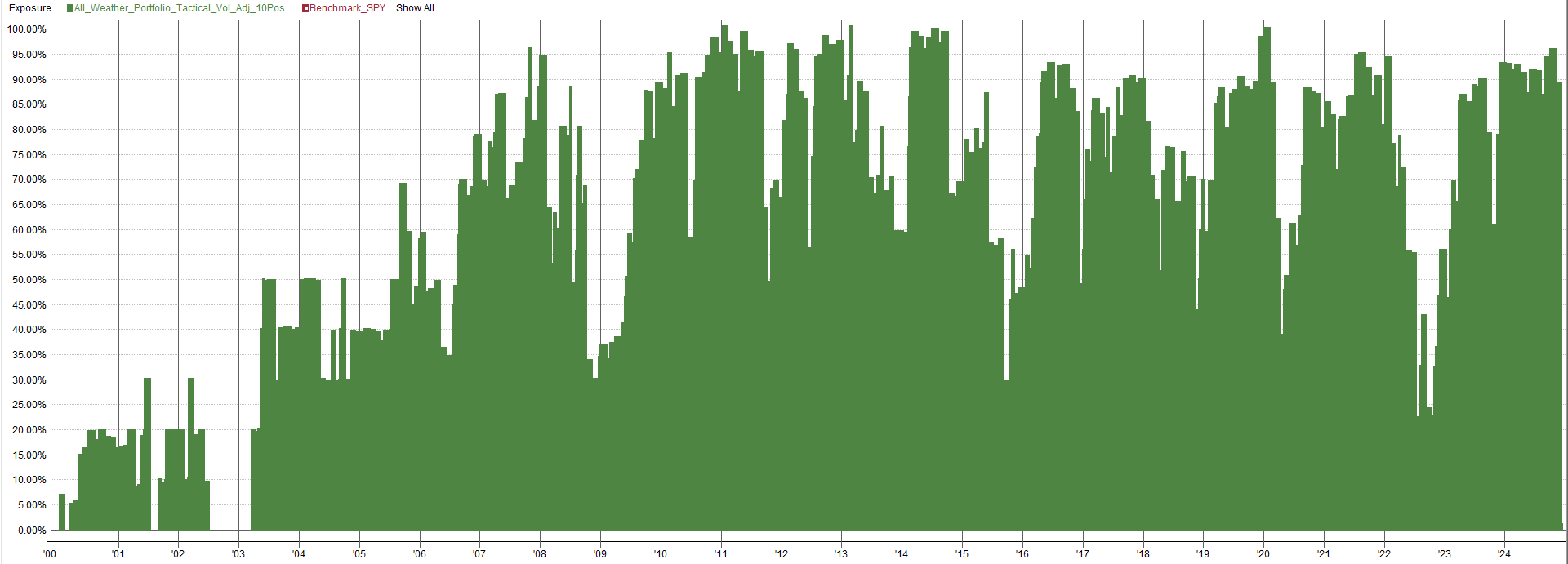
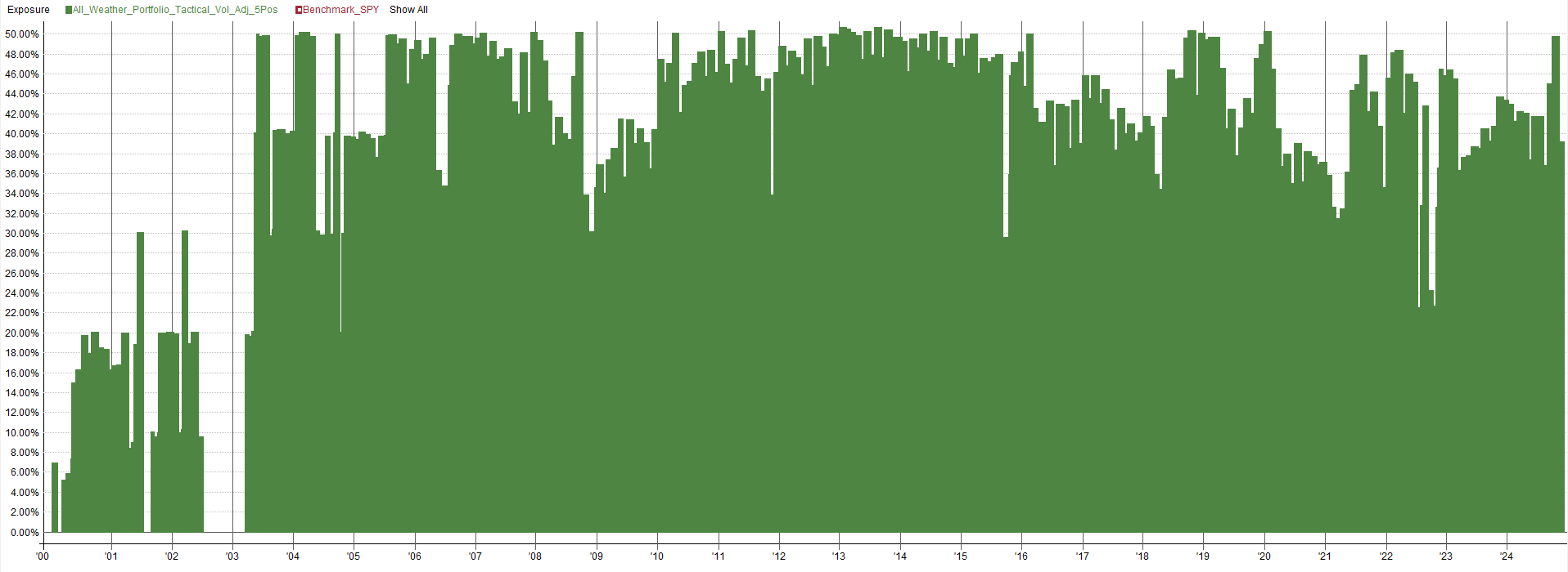
Though maybe you want more than a 6% return. Maybe you are the type of person who is okay with more volatility in exchange for a more returns. Well there is a solution for that. To increase the returns we have to give something up, in this case we will give up diversification. Instead of holding 10 positions, we will hold 5 positions. Just holding 5 positions though would lead us to be under exposed with a max exposure of 50%, see below:

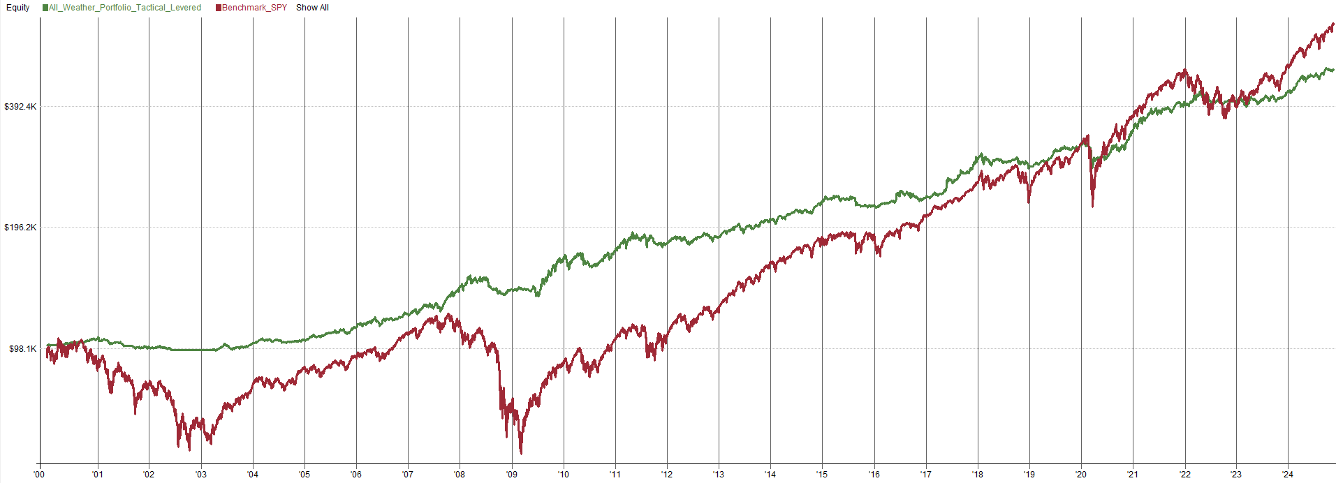
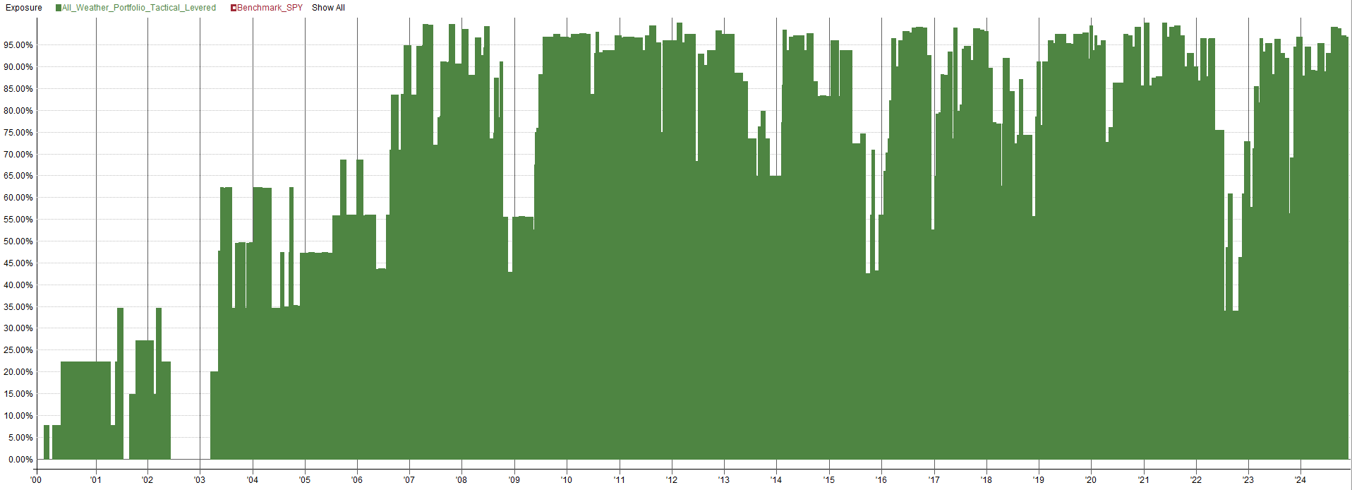
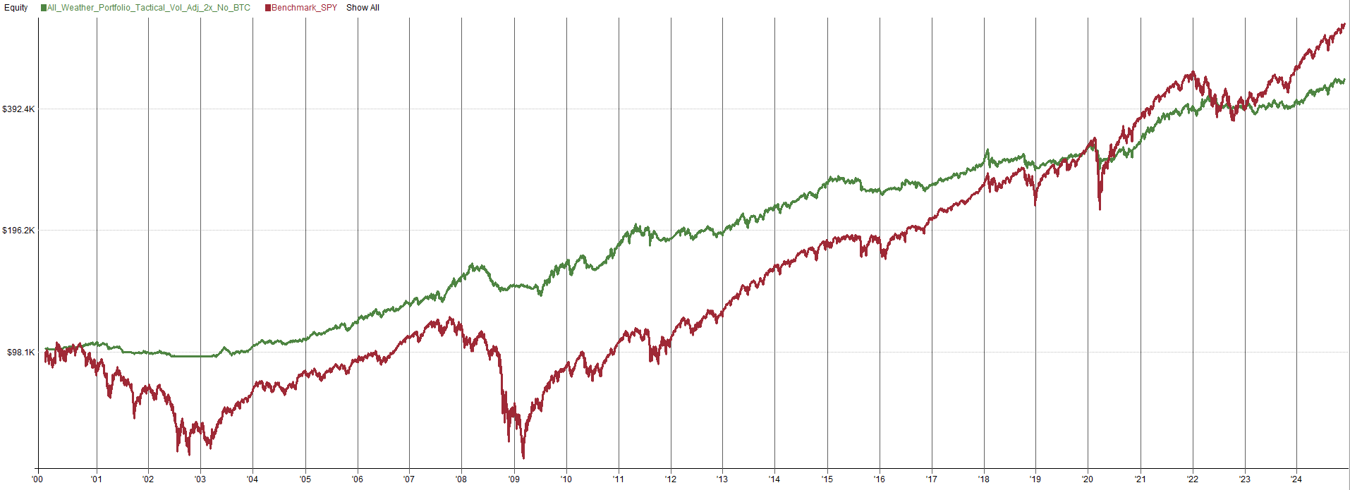
As you can see, just reducing from 10 to 5 positions leads to less returns because we only use half the money. So, we are then going to double the position size, to fully utilize all the capital with the 5 positions. See below for an equity curve of the final third All Weather portfolio with 5 positions and 2x the position size of the 10 position All Weather portfolio:

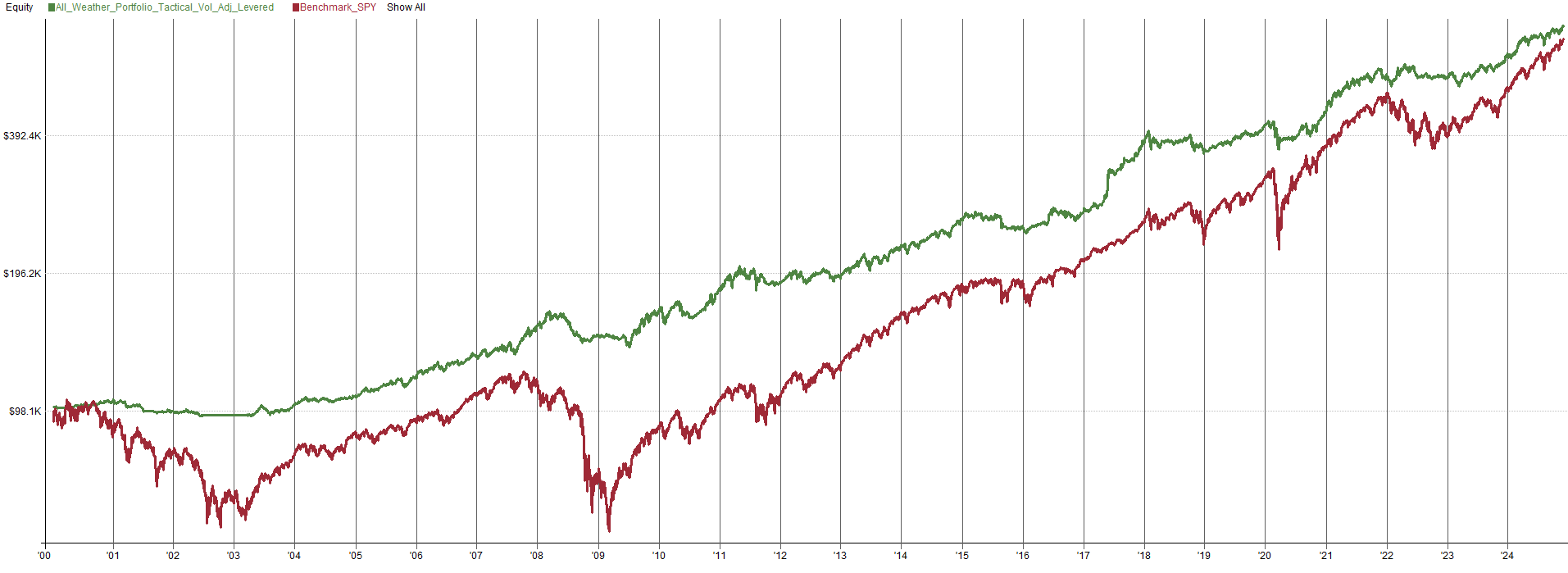
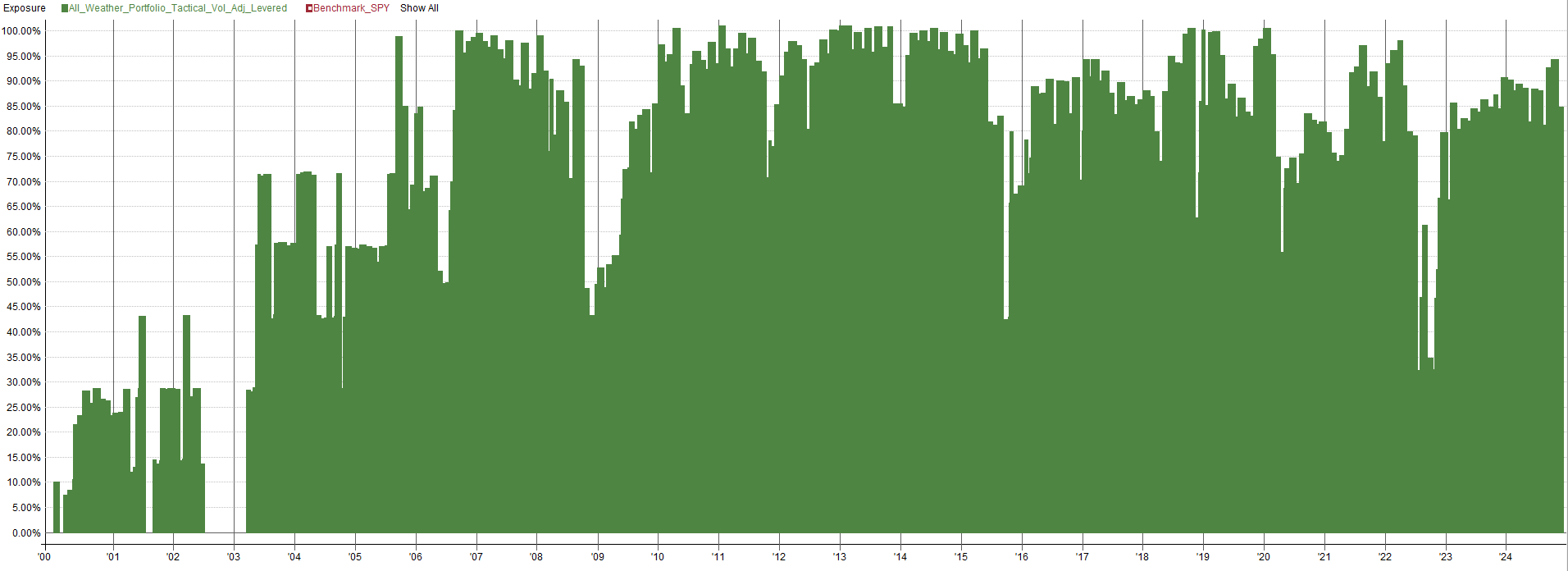
This levered up model achieves higher returns, but experiences more volatility and drawdown. Depending on your objectives that may be fine, but nothing comes for free, if you want higher returns you have to accept more volatility. Pretty wild how such a simple model can beat SPY over the long run in terms of returns and has less than 1/3rd the drawdown of SPY. This system beats SPY on both an absolute level and risk adjusted level. Sure, there will be some points in time where this All Weather portfolio will underperform SPY, that’s life, we can’t always win; but considering what this All Weather portfolio has done over a 5 to 10 year timeframe, I’ll take it.

One thing you may be thinking is how there is a spike in the equity curve in 2017. Well that’s Bitcoin, it was so volatile that a one month rebalance period was not sufficient enough to dampen the volatility. Below is the performance without Bitcoin, which is still very good.

This type of system could be a great option for someone looking to build wealth with less downside risk. I personally plan to implement this strategy into my arsenal of many trading systems. I like the diversification it provides as this system was intentionally designed to trade mostly uncorrelated ETFs. I do not have any other systems like this, so I am excited to add a new income stream to the portfolio.

One thing to consider. While I am comparing these All Weather portfolios to buy and hold SPY ETF, I have not accounted for taxes. There may be situations where the tax implications of having a tactical trading approach may not make sense. Taxes are different from state to state and country to country, I would never be able to model taxes in a way that was applicable to everybody. So just keep that in the back of your mind with these results.

Conclusions:

In this article we looked at three versions of All Weather portfolios, with a couple different variations along the way. The first All Weather portfolio was buy and hold all ETFs with periodic rebalancing based on a static capital allocation calculated from the average volatility of the ETF. The second All Weather portfolio used the same position sizing method, but introduced a tactical asset allocation where we only own an ETF if it is trending up. The third All Weather portfolio used the same tactical asset allocation, but used volatility based position sizing that is adjusted over time, rather than a static allocation. This just goes to show that simple can be effective. We don’t need super complex fancy trading systems to get good returns.

There is actually one more All Weather portfolio I want to explore that takes the result one step further. So, yes that means there will be a part three to this series. What I will do is start with the third All Weather portfolio and look at more frequent rebalancing periods to reduce the volatility and drawdown of the portfolio even further. So keep in mind the part 3 article is coming in the next few weeks. So seen you then!